Keeping up with the times: DSP-based receiver for ALS162 - Part 2

TLDR:

In this series I am exploring the idea of building a DSP-based receiver for ALS162. The last entry covered the hardware and general design aspects. In this one I will go over the software/firmware side of things.

For the first prototype I made I chose an STM32 microcontroller, more specifically the STM32L476RETb. I’m using STM32CubeIDE and the provided “HAL” libraries to program the microcontroller. The second revision board I’m showing here has a different format and some minor changes, but the working principles remain untouched.

Sampling

First things first. Any DSP system starts with converting an analog signal into a digital one. This is a job for an Analog-to-Digital Converter (ADC). As was discussed in the last chapter, we must sample at least at 1 Msamples/s.

Timers and clocks

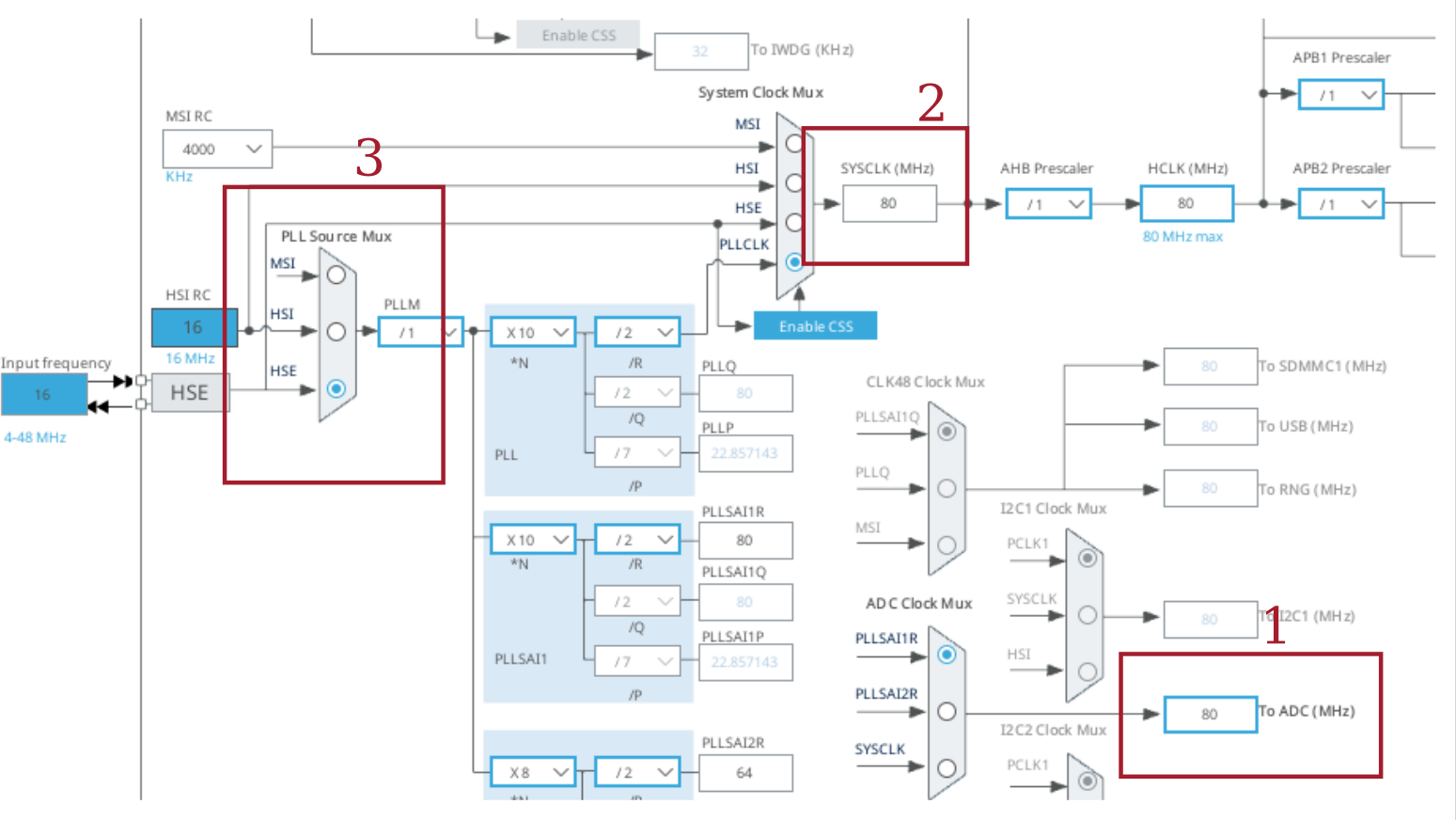
To achieve the desired sample rate, we must firstly change some parameters in the “Clock Configuration” tab.

1. The ADC clock source is configured to 80 MHz, otherwise the ADC won’t be able to sample at the necessary speed.
2. The system clock is configured to 80 Mhz (nominal)
3. The PLL source mux is configured to use the external high-speed crystal (HSE). This will become important later on.

This is made easy with the integrated CubeMX code generator in STM32CubeIDE, as it reconfigures the various dividers and multipliers to achieve the desired frequencies.

Afterwards, a timer is configured such that it triggers a conversion of the ADC at a rate of 1 Msamples/s (Fadc). To achieve this, the prescaler (PSC) and autoreload register (ARR) are configured such that:

$$ F_{ADC} = \frac{F_{CLK}}{(PSC+1)(ARR+1)} $$

For Fadc = 1 MHz and Fclk = 80 MHz one can choose the following values: PSC = 79; ARR = 0. Then the timer trigger out (TRGO) is configured as “Update Event”. This triggers the output on counter overflow (i.e., at 1 Msps).

ADC, DMA

Because the ADC will sample at such high speeds, conversions are triggered directly by the timer that was configured before, and the result of that conversion is copied to memory via Direct Memory Access (DMA). This allows the sampling to happen with virtually zero CPU time required.

Some bits have to be configured in the ADC, the most important of which is the external conversion trigger, which will start a sample on every tick from the timer

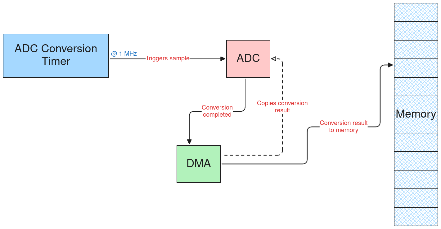
The DMA1 peripheral is configured in Peripheral-to-Memory operation (pretty self-explanatory) and circular mode. This last setting means that the peripheral runs continuously, wrapping around the target buffer.

Ping Pong

The main advantage of using the DMA peripheral is that the CPU is not involved in fetching the results. However, this also means that the CPU doesn’t know where or when the DMA is writing new data. To be able to work together, a so-called “ping pong” buffer is frequently used.

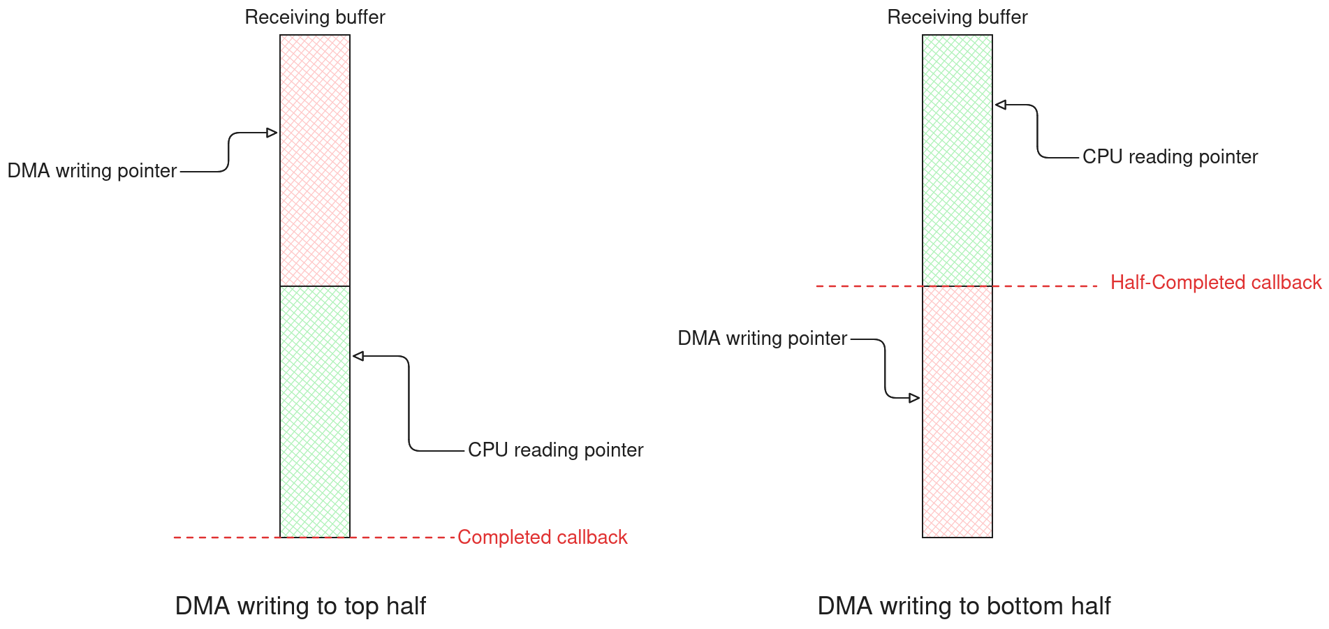
In this configuration, a buffer double the intended batch size is created. Then, the DMA peripheral is configured to invoke two callbacks

• One when half of the buffer has been filled
• One when the whole buffer has been filled

This way, the CPU can work on a completed batch of results (one of the halves of the buffer) while the DMA writes to a buffer containing the next batch (the other half), with no overlap or race conditions. W

I/Q Demodulation

Now the signal exists as its digital representation. This signal is the raw modulated carrier; to extract any useful signal this signal must first be demodulated.

How it works

I/Q demodulation achieves this by mixing the input signal with two sinusoidal signals π/2 radians out of phase. For continuous signals, when a signal with a phase given by ωt+ θ is multiplied with an oscillator with angular frequency Ω, and remembering basic trigonometric properties $$ S = A\cos(\omega t + \theta) $$

$$ S \cdot \cos(\Omega t) = A\cos(\omega t + \theta) \cdot \cos(\Omega t) = A \cdot \frac{cos[(\omega+\Omega)t + \theta]+ \cos[(\omega - \Omega) t + \theta]}{2} $$

Firstly, it can be observed that the signal resulting from this operation has two frequency components:

• The sum of the angular frequencies
• The difference of the angular frequencies

Secondly, if the high-frequency component is eliminated (perhaps through a low-pass filter), what remains is $$ A \cdot \frac{\cos[(\omega - \Omega) t + \theta]}{2} $$ Here θ measures the relative phase offset between receiver and transmitter; it’s trivial to see then that if our oscillator had a π/2 radian offset, the resulting phase offset value would also be shifted π/2 radian. Knowing that cos(θ-π/2)=sin(θ), it’s trivial to see that if $$ I = \left[ S \cdot \cos(\Omega) \right] \vert_{low-pass} $$

$$ Q = \left[ S \cdot \cos(\Omega + \pi/2) \right] \vert_{low-pass} $$

Then $$ \frac{Q}{I} = \tan((\omega-\Omega)t + \theta) $$ If, additionally, the frequency of the oscillator is matched to that of the carrier, then the phase difference between the receiver and the transmitter can be obtained, effectively demodulating our phase-modulated signal.

Overview and main components

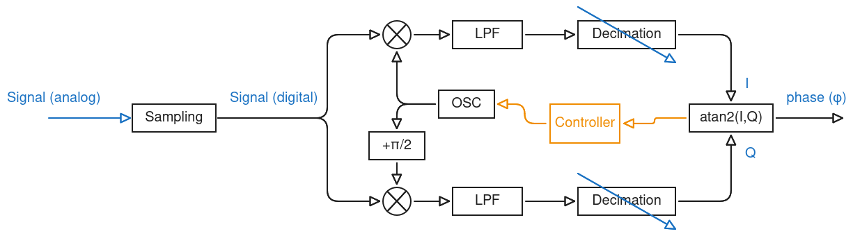
The basic steps to implement i/q demodulation are shown in the following diagram.

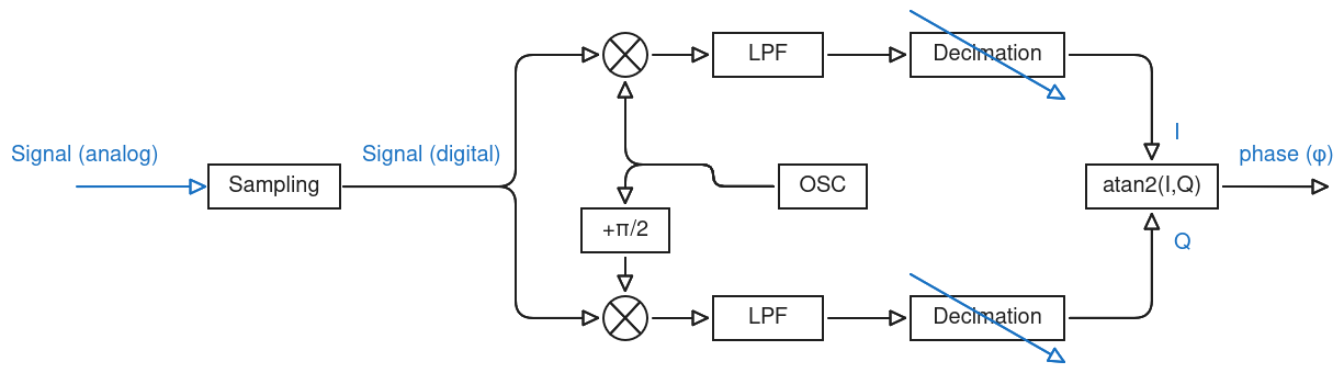
The two circles represent the multiplication operation (or “mixing”) shown before. They are followed by a low-pass filter to remove the high frequency components. Decimation afterwards is not strictly necessary, but as the signal has now been shifted to the baseband it’s convenient to work with a lower sampling rate, as less samples means less computational resources needed.

Mixing

The first part to implement is the mixing of the signals. For performance reasons it’s best to bunch as many samples together as possible. Let’s say for now that the filter will later have a decimation ratio of 1000; this means that every 1000 samples on the input it would produce 1 sample on the output. In this configuration, samples would need to be processed in groups of at most 1000 samples to maintain the cadence on the output side.

The main concern with mixing is that the input sample rate is so high that the number of cycles/sample is very limited. For this reason, both the trigonometric functions and the actual multiplication need to be very optimized.

A fast numerical oscillator

To generate the cos(x) and sin(x) I used a numerically controlled oscillator (NCO). An NCO consists of two fundamental parts

• A phase accumulator
• A phase-to-amplitude converter

For the phase accumulator I used a 32-bit number. The maximum value of the number represents 2π. The phase accumulator is advanced (i.e., a number is added to it) every sample (i.e., at fs = 1 MHz), meaning that if the number must overflow at a frequency fnco, the value to be added each sample would be: $$ \text{Phase Difference} = \frac{f_{nco}}{f_s} \cdot 2^{32} $$ The phase-to-amplitude converter is more critical performance-wise. There are various ways to implement it, but perhaps the fastest is using a lookup table (LUT). If we used the whole phase accumulator as an index into the LUT, the resulting LUT would be monstrous (2^32 entries, or slightly more than 8 gigabytes of memory at 2 bytes/entry), so instead only the top n bits are used.

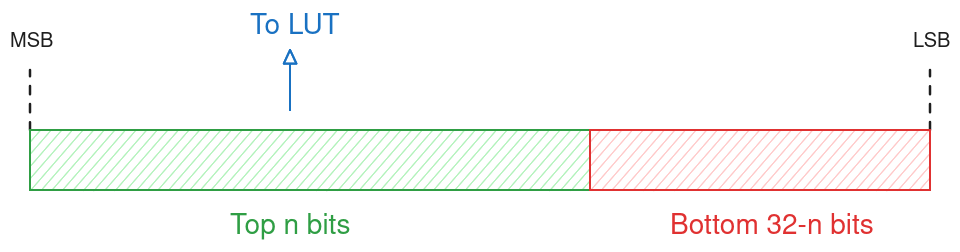
This arrangement is quite clever, because the phase lookup table can be rather small (limited resolution), but the fact that the phase accumulation is done on the full resolution of the accumulator means that the “average” frequency can be set with a high degree of granularity. Of course, the signal will have some jitter due to the quantization error during each lookup, but this is not noticeable in this application.

Only one table is needed to compute cos(x) and sin(x), as $$ \cos (x-\pi/2) = \sin(x) $$ Therefore, if only the table for cos(x) is available, we can subtract the equivalent to π/2 from the accumulator (x) and get the index corresponding to sin(x).

Fast multiplication

The next step to get a mixed signal is to compute the product of the oscillator and the input signal. To achieve the fastest speeds, the incoming integer value is scaled to a Q1.15 fixed-point number, the bias voltage is extracted, and the two products are computed using fixed-point formats. Then, both are stored into a 32-bit buffer.

/* Local phase accumulator to allow for better compiler optimization */
uint32_t phase = hfreq_phase_accumulator;
uint32_t phaseInc = hfreq_phase_difference;

for (uint16_t i = 0; i < CONF_SAMPLING_HFREQ_BUF_SIZE; i++) {
    // Bias and scale in Q15
    q15_t samp = ((q15_t)in_buf[i] << 3) - vbias_q15;

    /* The top 15 bits of the phase accumulator are used to access the LUT */
    /* For the sin table we exploit that cos(a + pi/2) = -sin(a), pi/2 being 2^15/4 in the LUT index */
    uint16_t idx = phase >> 17;
    q15_t mycos = cos_lut[idx];
    q15_t mysin = cos_lut[(idx + 8192) & 0x7FFF];

    /* Multiply into 32 bit register, then shift back to 16 bit */
    /* The NCO is adapted so that the minimum value is -32767, so
     * the fixed point multiplication can never overflow. Therefore,
     * no saturation needed */
    q15_t cos_val = (q15_t)(((int32_t)mycos * samp) >> 15);
    q15_t sin_val = (q15_t)(((int32_t)mysin * samp) >> 15);

    /* Store samples into the dual buffer to be fed to the DFSDM */
    dual_buf[i] = ((uint32_t)(uint16_t)sin_val << 16) | (uint16_t)cos_val;

    // Advance phase
    phase += phaseInc;
}

hfreq_phase_accumulator = phase;

While the STM32L476 does have a single-precision FPU, using fixed-point arithmetic avoids costly integer-to-float and float-to-integer conversions. To use fixed-point arithmetic the LUT must also be computed and stored in the same Q1.15 format.

Generally, fixed-point multiplication of two 16-bit numbers entails the following steps:

• 32-bit multiplication of the two 16-bit values.
• Saturation.
• Rightwards shift.

The saturation is necessary because two’s complement-codified numbers do not have a symmetrical range from zero; a signed m-bit integer can represent a number from -2^(m-1) to 2^(m-1)-1. In a Q1.15 format, this would mean a range from -1.0 (0x8000) to +0.99997 (0x7FFF), thus, if one were to try -1.0 * -1.0, the resulting number (+1.0) would overflow the register. To avoid this edge case, the LUT is computed saturating to -0.99997 (0x8001), thus eliminating the need for saturation.

Other tricks used to further enhance the performance of the loop are:

• Caching the phase offset and phase accumulator into local variables, to allow for more aggressive compiler optimization.
• Using a sum + mask instead of a sum+shift to compute the access for the sin(x).

Care is also taken to force the compiler to optimize the section for speed through the following GCC directive:

#pragma GCC push_options
#pragma GCC optimize ("Ofast")

A performance problem

Once mixing has been performed, the sample has to be low-pass filtered and decimated. Taking into account the CPU time used by the mixing process, only 40 cycles/sample are still available, and we must take into account that the decoding step and other auxiliary processes might use a significant portion of that available CPU time, so the filtering step should use no more than 20 cycles/sample.

Even with highly optimized algorithms using single-cycle multiply-accumulate instructions, it’s very difficult to stay within this performance budget.

DFSDM

The answer to this performance issue is also the reason I chose this particular microcontroller: the so-called STM32 Digital Filter for Sigma-Delta Modulators (DFSDM). This peripheral is designed to receive a PDM bitstream and low-pass filter it down to recover the original signal (downsampling/widening samples).

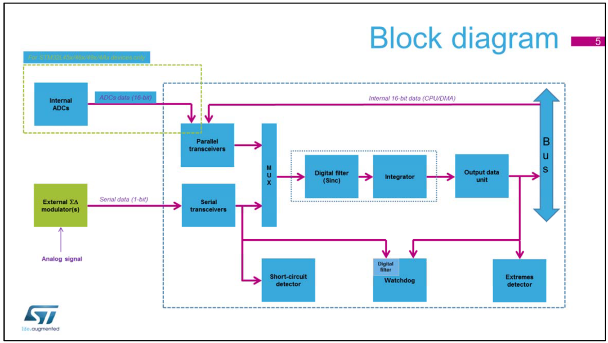
However, as the marketing material shows, the DFSDM is quite flexible and can also take in any arbitrary signal (not only bitstreams) through parallel inputs. Thus, we can use it to replace the LPF+decimation blocks seen on the diagram.

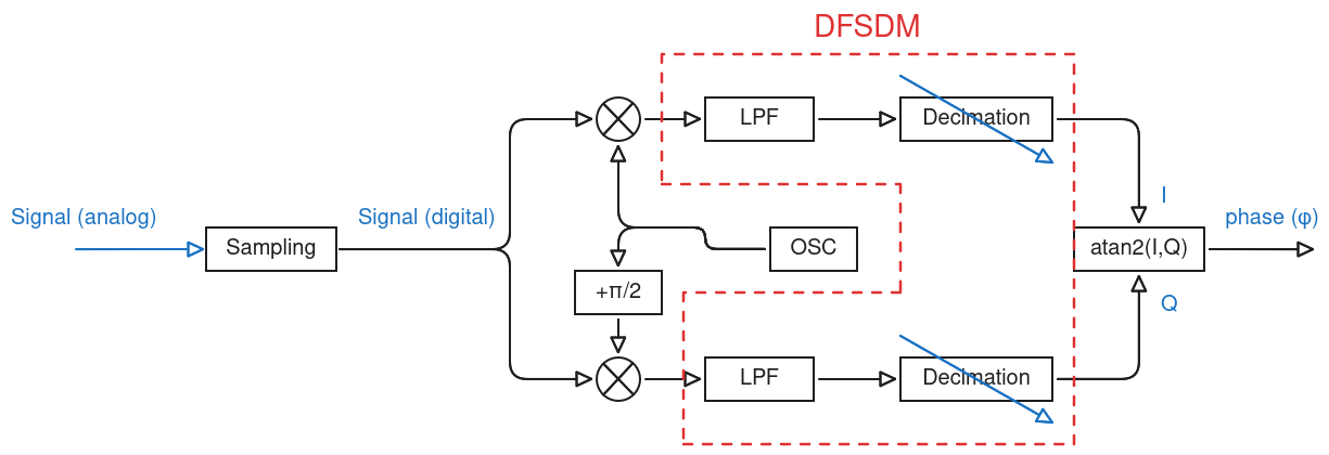
Fundamentally, the DFSDM contains a configurable cascaded integrator-comb (CIC) filter, a type of finite impulse response (FIR) digital filter.

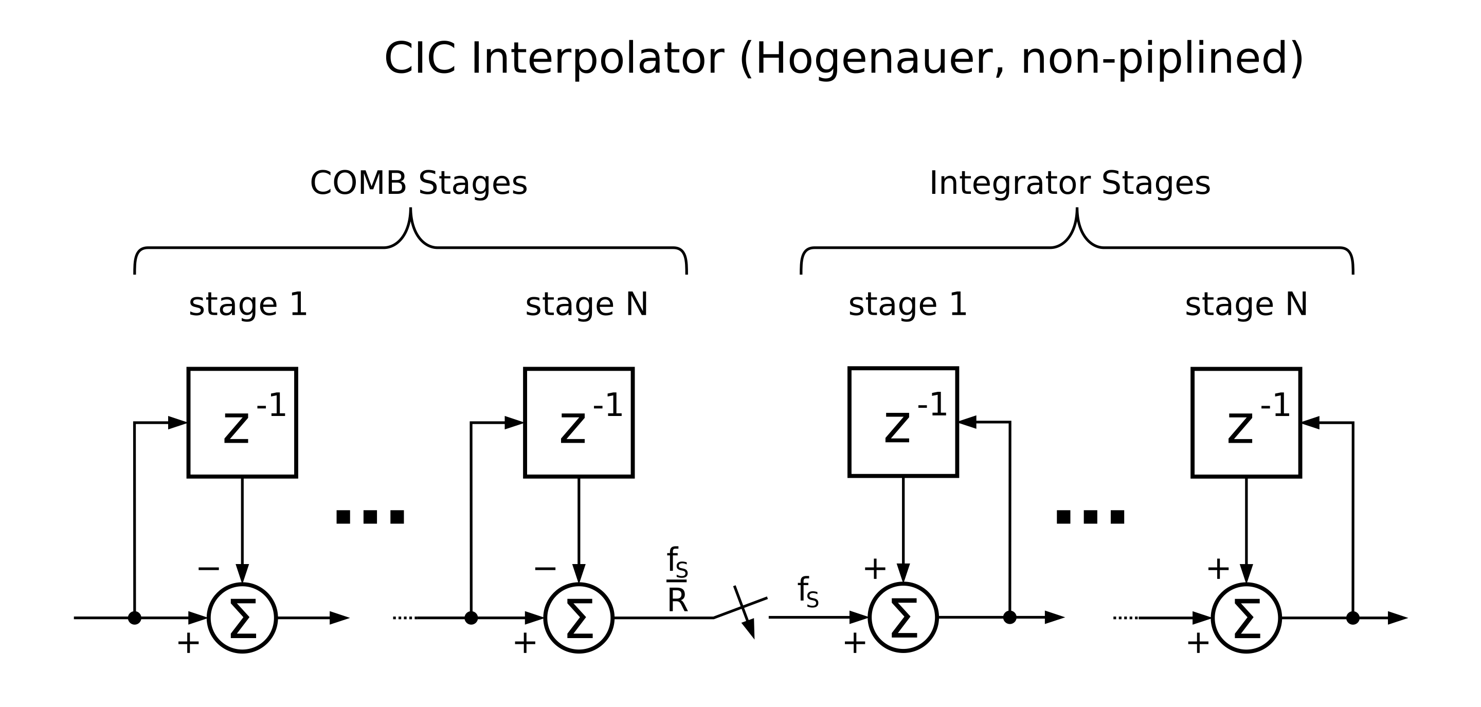
The CIC filter is interesting for this case because the filter has an integrated decimator (a decimator discards all but 1 our of R samples). I will not discuss the technical details of CIC filters, but there are some important parameters to be aware of:

• Filter order (N): how many stages are chained
• Decimation ratio (FOSR): the signal is downsampled by FOSR.

The DFSDM implementation also includes an additional “integrator unit”, which sums IOSR samples into one final output sample. However, as will be seen shortly, it’s not very useful for this application.

Understanding the DFSDM

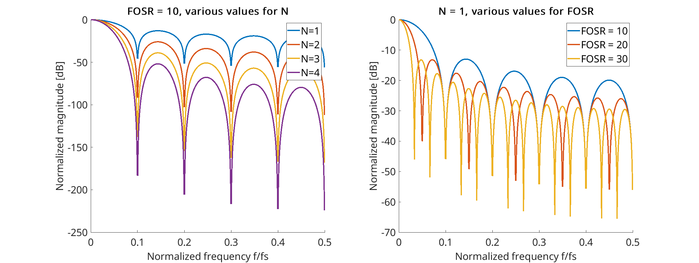
As the DFSDM is being used as a low-pass filter, one obvious design criterion is for the filter to be “as good as possible”. In this regard, the transfer function is an interesting starting point: $$ H(z) = \left( \frac{1-z^{-FOSR}}{1-z^{-1}} \right)^N $$ The Bode magnitude plots of various FOSR and N configurations clearly show the effects of both parameters on the transfer function.

• Generally speaking, the higher the filter order (N), the sharper the roll-off and the higher the stop-band attenuation.

• FOSR also makes the filter slightly more aggressive, but it’s important to remember that FOSR affects the output sampling rate. Therefore, it’s not a fully independent parameter.

One thing to take into account is that these plots are normalized for magnitude. However, CIC filters have a certain gain, which results in bit growth (more bits are required to represent a sample). This is how a bitstream grows into a multi-bit number, for example. The bit growth of a CIC filter is given by: $$ \text{Bit Growth} = \lceil N \cdot \log_2 (FOSR) \rceil $$ The maximum width of the peripheral must not be exceeded; this gives us another constraint.

Final configuration

For this project I chose a value of FOSR = 1000, such that for an ADC sampling frequency of fs = 1 MHz, the sampling rate on the output is: $$ f_s^{’} = \frac{f_s}{FOSR} = 1000 \ \text{Hz} $$ Or one tick every 1 ms. This will make decoding easier, as the demodulated signal contains patterns that can be easily represented with a 1 ms time base.

The filter order is limited by the allowed bit growth. Given that the ADC has a resolution of 12 bits and an internal resolution of 31 bits, the maximum allowed bit growth would be of 19 bits. So, for example, for N = 2: $$ \text{Bit Growth} = \lceil N \cdot \log_2 (FOSR) \rceil = \lceil 2 \cdot 9,966 \rceil = 20 $$ The options here are to either reduce the filter order to N = 1 or to ensure that the input stays below a certain value (+-1073). Both options are valid; it’s a trade-off between better filter frequency response and potentially lower quantization noise. In practice the analog signal is always kept well clear of the limit, as RRIO op-amps can behave non-linearly when pushing the output, so I have used N=2

It’s easy to see that if the maximum resolution becomes a constraint then an additional integrator block (which would add more bit growth) is not of interest. For this reason I set IOSR = 1.

Computing the phase

The mixed signal is fed to the DFSDM and what comes out is a stream of I and Q values at 1000 Hz (1 sample every millisecond). As discussed before,

$$ \frac{Q}{I} = \tan((\omega - \Omega)t+ \theta) $$ Therefore, to get the phase difference between the input signal and the local oscillator, the program only needs to take the arctangent of Q/I (or more programatically, to take atan2(Q, I)).

Closing the loop

The phase value obtained before is only useful if the frequency difference between the carrier and the local oscillator is reduced to zero. In practice, a quartz oscillator has accuracies in the order of tens of ppm of initial accuracy by themselves, and this margin is further increased by parasitic load capacitances on the board.

To compensate for this deviation, a common solution is to “close the loop”, that is, to place a controller that adjusts the local oscillator based on the phase difference. What we want to achieve, essentially, is to filter out the part of the signal corresponding to the frequency difference.

There is a problem with this idea, however. If we visualize the problem in the frequency domain, it essentially has two groups of components: those corresponding to the signal of interest (which sit around the baseband, and up to ~6.3 Hz) and those corresponding to the frequency gap (a narrow spike anywhere from 0 to 20 Hz):

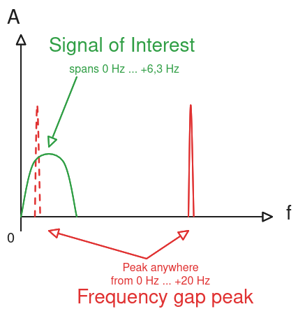
Filters are usually characterized by their frequency response; however, in this case we do not know where in the frequency spectrum the “unwanted” spike will be, we cannot discern between wanted and unwanted components based on their frequency.

A two-step approach

To fix this, I try to approximate the frequency error by opening the loop and running an Fast Fourier Transform (FFT) on the signal. The peak corresponding to the frequency error is stronger than the actual signal, so the code can approximate how offset our crystal really is from the FFT results.

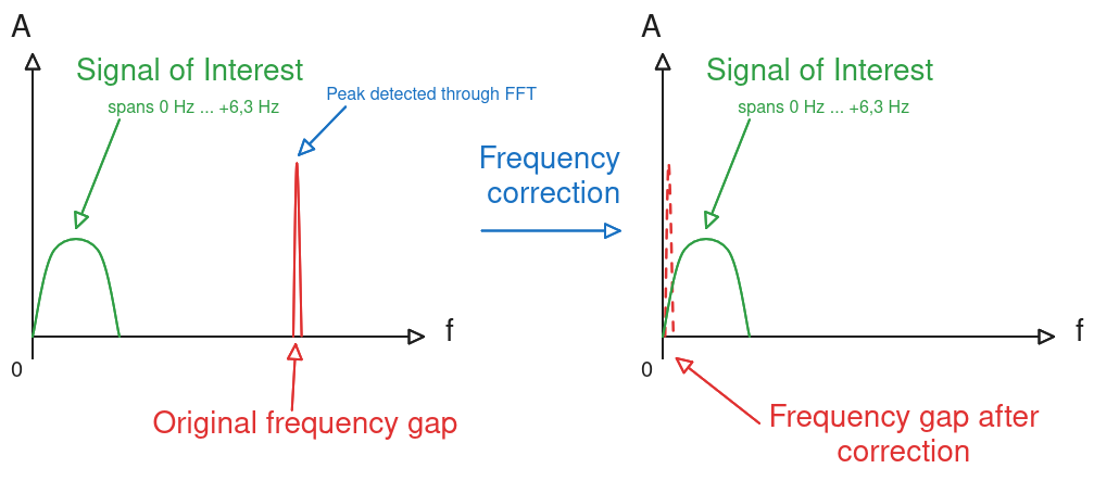
The crystal is now calibrated so that the difference between the local oscillator and the emitter is approximately zero. The FFT gives us a value with a resolution of about +-1 Hz. Because of this, if we look the actual signal, we see that there is still a very low-frequency component present.

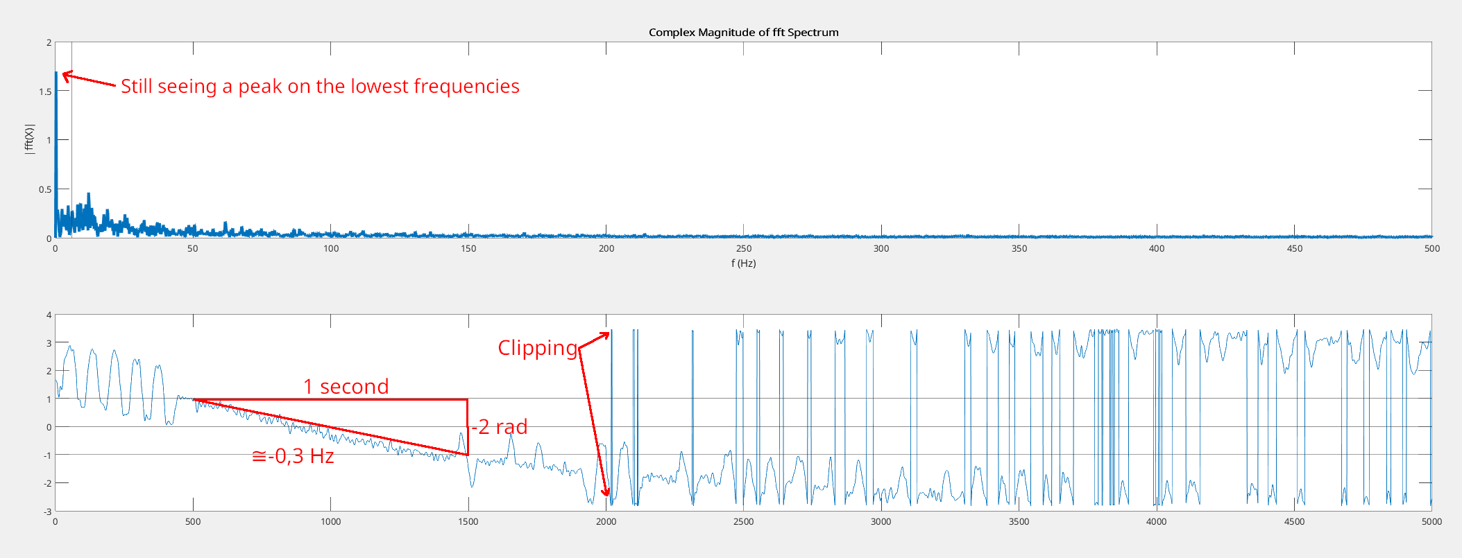
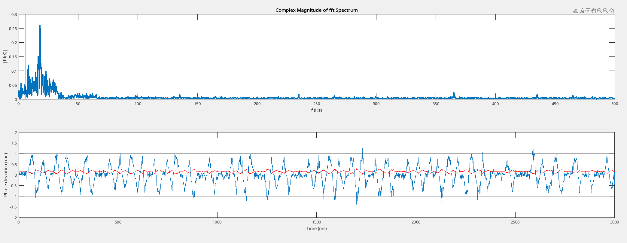
We can now go back to the old “closing the loop” idea and implement a sort of phased-locked loop, because we now know that we want to remove only the lowest frequencies (<1 Hz). I implemented a simple PI controller in software that adjusts the phase difference of the oscillator as a function of the phase; by altering its constants we can change the frequency response of the whole loop.

static inline void updatePll(float v) {
	float e = -v;
	i_acc += e * 0.001f;
	pll_out = conf_pll_kp * e + conf_pll_ki * i_acc;
	uart_debug_2 = pll_out;
	hfreq_phase_difference = FREQ_OFFS_TO_PHASE_DIFF(-crystal_offs - pll_out/(float)M_2_PI);
}

After a bit of manual tweaking, the loop locks correctly and the signal is now nice and centered

Decoding

It’s now time to start decoding the signal. As you may have noticed on previous screenshots, the noise level on the signals is quite considerable. This is not due to my hardware but because the signal is very weak and quickly drowns below the noise floor on noisy environments, such as a room with multiple switching converters and other electronic devices.

The signal only uses one pattern to represent symbols: an upwards ramp to +1 rad during 25 ms, then a downwards ramp to -1 rad during 50 ms and an upwards ramp again to 0 rad during 25. Each second, either one or two of these patterns is transmitted, with one pattern meaning “0” and two back-to-back patterns meaning “1”.

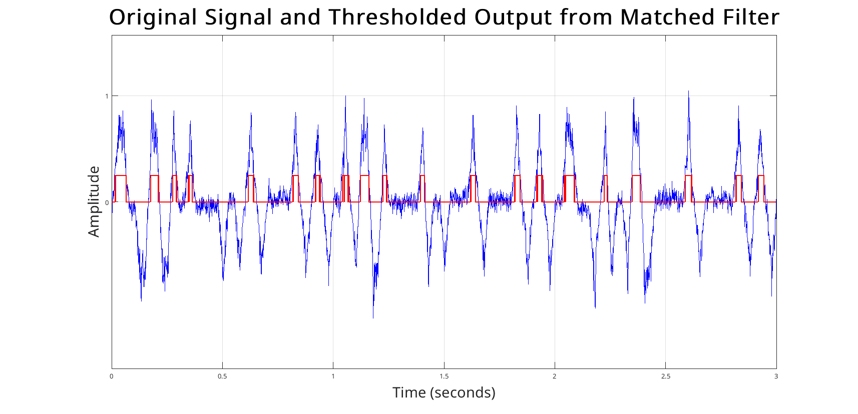
To maximize the sensitivity of the receiver, I implemented a so-called “matched filter”, which is a type of filter that is often used to find a delayed version of a known signal. It’s essentially a moving correlation of the signal with a template of the pattern to find. This video shows some nice animations of a matched filter in action

By running a matched filter and then thresholding, we can turn ramps into ones and zeros that indicate whether a pattern is present. I’ll call this signal the bitstream, as it contains only ones and zeros.

Synchronizing

To correctly interpret the bits we need to sync to the second markers. This is easier said than done, because time data is only part of the signal. From UTC second+200ms to the next UTC second, the signal encodes different data, whose format is not publicly available. The encoding is similar enough that we may match a pattern to it. This makes it tricky to synchronize to the actual, time-data bits.

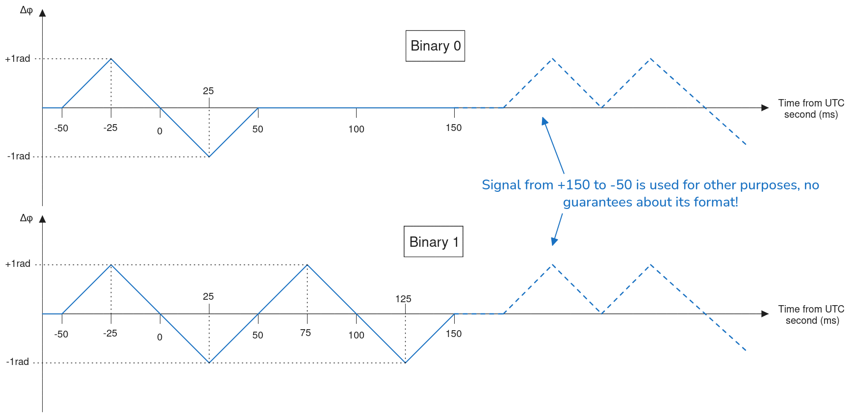
Fortunately, the last second of the hour contains no modulation at all during 1000 ms, which is very easy to spot. We can use this to synchronize to both the minute marker and the second marker.

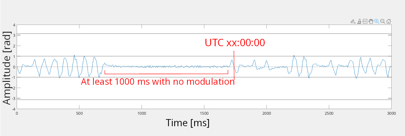
From here, the decoding process is quite simple: we first sync to the minute and second marker; then, when a pattern is expected, we check the bitstream. By evaluating the results we can check whether a logical “0” or “1” has been transmitted, and we fill a buffer with the results. Finally, we reconstruct the time data from the bits and check the parity conditions. If the parity conditions are satisfied, we’ve officially received time from the Allouis transmitter.

The results

Below is a short video showing the receiver in action. Note the following:

• Reception starts at the start of the minute. After the minute sync, an LED starts flashing as bits are received.
• After 1 complete minute, the receiver updates the time and displays it on the screen.
• The time (1 AM). This is because there is less electromagnetic interference at night, which increases the quality of the received signal.

To conclude this project, I have demonstrated that it is possible to receive, demodulate, and decode the ALS162 signal using nothing but a few off-the-shelf components, by taking advantage of DSP techniques and modern microcontrollers. I estimate the BOM cost of the board to be around 15€, much less than what a specialized receiver or SDR setup would cost.

PS: I have no intention of developing this project any further. If you have any questions feel free to ask - I’ll be glad to answer them!